2D Convolution Calculator: Visualize Image Processing Operations

How to Use the 2D Convolution Calculator Effectively

The 2D Convolution Calculator is a powerful tool designed to perform convolution operations on two-dimensional matrices. To use this calculator effectively, follow these steps:

1. Select Input Matrix Size: Choose the dimensions of your input matrix from the dropdown menu. Options include 3×3, 5×5, and 7×7. For example, select 5×5 for a medium-sized input matrix.
2. Choose Kernel Size: Select the size of your convolution kernel. Options are 3×3 and 5×5. For instance, choose 3×3 for a compact kernel.
3. Set Padding Type: Select the type of padding to apply to the input matrix. Options include:
   • None: No padding is applied
   • Zero: Pad the input with zeros
   • Reflect: Pad by reflecting the edge values
   • Replicate: Pad by repeating the edge values
   For example, choose “Zero” padding to maintain the input size.
4. Specify Stride: Enter the stride value, which determines how the kernel moves across the input matrix. A common value is 1, but you can experiment with larger values like 2 or 3 for downsampling effects.
5. Select Convolution Mode: Choose from “Valid,” “Same,” or “Full” convolution modes. For instance, select “Same” to maintain the input matrix dimensions in the output.
6. Input Matrix Values: Fill in the values for your input matrix. For a 5×5 matrix, you might enter values like:
   1 2 3 4 5
   6 7 8 9 10
   11 12 13 14 15
   16 17 18 19 20
   21 22 23 24 25
7. Kernel Matrix Values: Enter the values for your convolution kernel. For a 3×3 kernel, you could use:
   -1 0 1
   -2 0 2
   -1 0 1
8. Compute Convolution: Click the “Compute Convolution” button to perform the calculation.
9. View Results: The result will be displayed in the output matrix below the form.

Understanding 2D Convolution: Definition, Purpose, and Benefits

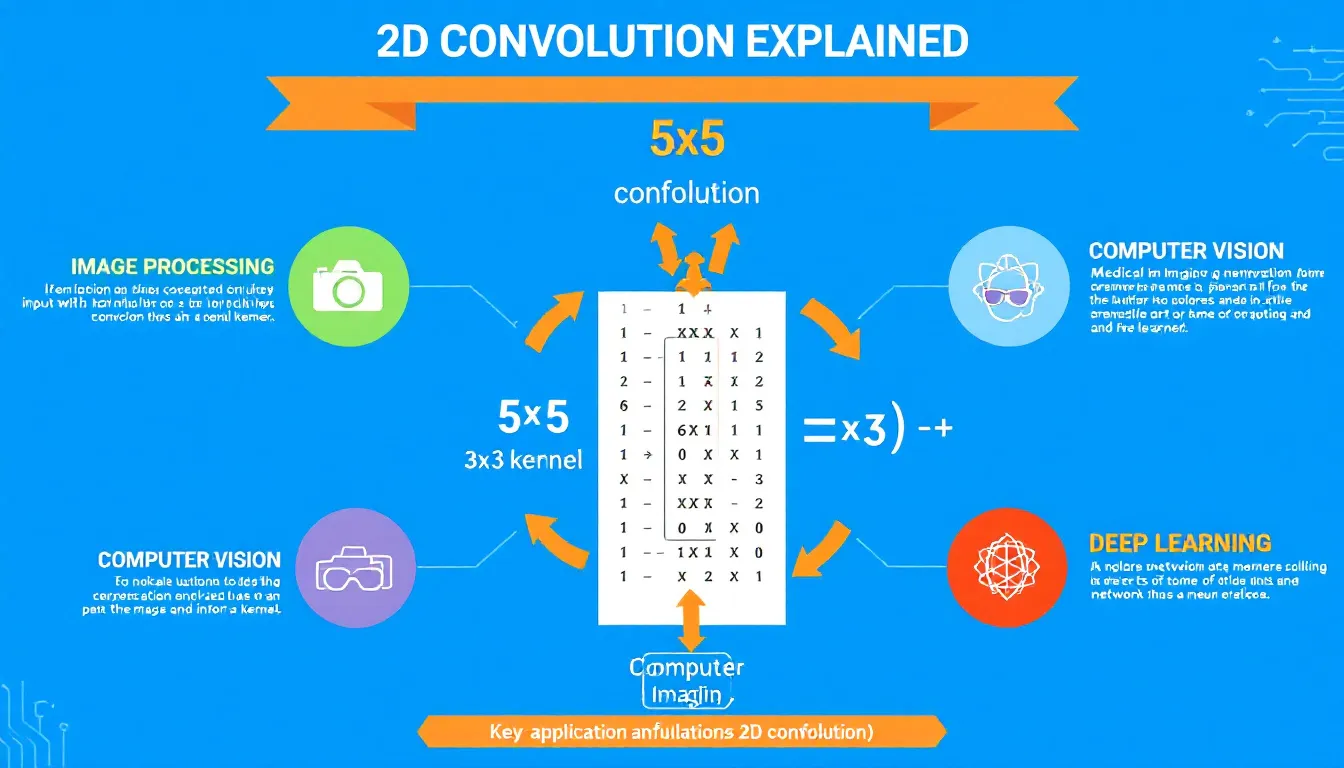
2D convolution is a fundamental operation in image processing, computer vision, and deep learning. It involves sliding a small matrix (kernel) over a larger matrix (input) to produce a new matrix (output) that represents transformed features of the input.

Mathematical Definition

The 2D convolution operation can be mathematically defined as:

Where:

• $$f$$ is the input matrix
• $$h$$ is the kernel matrix
• $$i$$ and $$j$$ are the coordinates in the output matrix
• $$k$$ is half the size of the kernel (assuming an odd-sized kernel)

Purpose of 2D Convolution

The primary purposes of 2D convolution include:

• Feature Extraction: Identifying important features in images such as edges, textures, and patterns.
• Noise Reduction: Smoothing images to reduce unwanted noise or artifacts.
• Image Sharpening: Enhancing details and improving image clarity.
• Blurring: Creating soft focus effects or reducing image resolution.
• Edge Detection: Identifying boundaries between different regions in an image.

Benefits of Using 2D Convolution

The benefits of employing 2D convolution in various applications are numerous:

• Spatial Context Preservation: Convolution operations maintain the spatial relationships between pixels, crucial for understanding image structure.
• Invariance to Translation: Convolutional filters can detect features regardless of their position in the image.
• Parameter Sharing: In neural networks, convolution layers use the same set of weights across the entire input, reducing the number of parameters and improving efficiency.
• Hierarchical Feature Learning: When used in deep neural networks, convolution layers can learn increasingly complex features as the network deepens.
• Versatility: The same convolution operation can be applied to various types of data, including images, time series, and audio signals.

Addressing User Needs and Solving Specific Problems

The 2D Convolution Calculator addresses several user needs and solves specific problems in image processing and machine learning:

1. Educational Tool for Understanding Convolution

Students and educators can use this calculator to visualize and understand the convolution process step-by-step. By inputting different matrices and kernels, users can observe how various filters affect the output.

2. Rapid Prototyping for Image Processing Algorithms

Developers and researchers can quickly test different convolution kernels without writing extensive code. This allows for faster iteration and experimentation in algorithm development.

3. Verifying Manual Calculations

The calculator serves as a reliable tool to check manual convolution calculations, helping users identify and correct errors in their work.

4. Exploring Padding and Stride Effects

Users can experiment with different padding types and stride values to understand their impact on the output dimensions and edge handling.

5. Demonstrating Convolution Modes

The tool allows users to compare ‘Valid’, ‘Same’, and ‘Full’ convolution modes, providing insights into how each mode affects the output size and border handling.

Example Calculations and Practical Applications

Example 1: Edge Detection

Let’s use the calculator to perform edge detection on a simple 5×5 image:

Input Matrix (5×5):

10 10 10 0 0
10 10 10 0 0
10 10 10 0 0
10 10 10 0 0
10 10 10 0 0

Kernel (Sobel operator, 3×3):

-1 0 1
-2 0 2
-1 0 1

Settings:

• Padding: Zero
• Stride: 1
• Convolution Mode: Same

Output Matrix:

0   0   60  0   0
0   0   60  0   0
0   0   60  0   0
0   0   60  0   0
0   0   60  0   0

This output clearly shows a vertical edge detected between the 10s and 0s in the input image.

Example 2: Blurring

Now, let’s apply a blurring effect to a 7×7 image:

Input Matrix (7×7):

0  0  0  0  0  0  0
0  0  0  0  0  0  0
0  0 100 100 100  0  0
0  0 100 100 100  0  0
0  0 100 100 100  0  0
0  0  0  0  0  0  0
0  0  0  0  0  0  0

Kernel (Gaussian blur, 3×3):

1/16 1/8 1/16
1/8  1/4 1/8
1/16 1/8 1/16

Settings:

• Padding: Reflect
• Stride: 1
• Convolution Mode: Same

Output Matrix (rounded to integers):

0   0   0   0   0   0   0
0  12  25  25  25  12   0
0  25  56  75  56  25   0
0  25  75 100  75  25   0
0  25  56  75  56  25   0
0  12  25  25  25  12   0
0   0   0   0   0   0   0

This result shows how the sharp edges of the original image have been smoothed out, creating a blurred effect.

Practical Applications of 2D Convolution

1. Image Enhancement in Photography

Photographers use convolution filters to sharpen images, reduce noise, or apply artistic effects. For example, a sharpening kernel might look like:

-1 -1 -1
-1  9 -1
-1 -1 -1

This kernel enhances edges and fine details in an image.

2. Medical Image Analysis

In medical imaging, convolution is used to enhance specific features in X-rays, MRIs, or CT scans. For instance, a Laplacian of Gaussian (LoG) filter can be used to detect edges in medical images:

0  0 -1  0  0
0 -1 -2 -1  0
-1 -2 16 -2 -1
0 -1 -2 -1  0
0  0 -1  0  0

3. Convolutional Neural Networks (CNNs)

In deep learning, CNNs use convolution layers to automatically learn features from images. While the kernels in CNNs are learned rather than predefined, understanding 2D convolution is crucial for grasping how these networks operate.

4. Satellite Image Processing

Geospatial analysts use convolution to process satellite imagery. For example, to detect urban areas, a kernel might be designed to highlight high-frequency changes in pixel intensity, characteristic of buildings and roads.

5. Computer Vision in Robotics

Robots use convolution operations in their vision systems to identify objects, detect obstacles, and navigate environments. Edge detection kernels are particularly useful in this context.

Frequently Asked Questions (FAQ)

Q1: What is the difference between convolution and correlation?

A1: Convolution and correlation are very similar operations. The main difference is that in convolution, the kernel is flipped both horizontally and vertically before sliding over the input, while in correlation, the kernel is used as-is. In practice, many implementations of “convolution” in image processing and deep learning actually perform correlation, as the flip operation doesn’t affect the learning process in neural networks.

Q2: How does the choice of padding affect the output?

A2: Padding affects both the output size and the treatment of edge pixels:

• No padding (“valid” convolution) reduces the output size.
• Zero padding helps maintain the input size but can introduce artificial edges.
• Reflect and replicate padding help maintain size while reducing edge artifacts.

Q3: What is the purpose of stride in convolution?

A3: Stride determines how the kernel moves across the input. A stride of 1 moves the kernel one pixel at a time, while larger strides skip pixels. Larger strides can be used to reduce the output size, similar to downsampling.

Q4: Can I use non-square kernels or input matrices?

A4: Yes, kernels and input matrices can be non-square. However, square matrices are more common in practice, especially in image processing and convolutional neural networks.

Q5: How do I choose the right kernel for my application?

A5: Kernel choice depends on the desired effect:

• For edge detection, use kernels with high contrast like Sobel or Prewitt operators.
• For blurring, use kernels with positive values that sum to 1, like Gaussian kernels.
• For sharpening, use kernels with a high central value surrounded by negative values.

Q6: What is the computational complexity of 2D convolution?

A6: For an input of size NxN and a kernel of size KxK, the time complexity of a naive 2D convolution is O(N²K²). However, more efficient algorithms exist, such as the Fast Fourier Transform (FFT) based convolution, which can reduce complexity for large inputs.

Q7: How does 2D convolution relate to 1D convolution?

A7: 2D convolution is an extension of 1D convolution to two dimensions. While 1D convolution is typically used for time series or audio data, 2D convolution is used for image data. The principles are the same, but 2D convolution operates over rows and columns simultaneously.

Q8: Can this calculator handle color images?

A8: This calculator is designed for single-channel (grayscale) images. For color images, convolution is typically performed separately on each color channel (Red, Green, Blue) and then recombined. However, you can use this calculator to understand the process for each individual channel.

Q9: What are separable convolutions?

A9: Separable convolutions are a special case where a 2D convolution can be broken down into two 1D convolutions (one horizontal, one vertical). This can significantly reduce computational complexity. Not all 2D convolutions are separable, but some common ones (like Gaussian blur) are.

Q10: How does this calculator handle floating-point precision?

A10: The calculator uses JavaScript’s native floating-point arithmetic. While this is sufficient for most educational and prototyping purposes, it may not match the precision of specialized scientific computing libraries. For high-precision applications, consider using dedicated numerical computing tools.

By understanding these concepts and utilizing the 2D Convolution Calculator, users can gain valuable insights into image processing techniques and develop a strong foundation for more advanced applications in computer vision and machine learning.